You are here: start » book » math » visdivcurl
Prerequisites
Visualizing Divergence and Curl
The Divergence Theorem says \begin{equation} \Int_{\rm box} \FF \cdot d\SS = \Int_{\rm inside} \grad\cdot\FF \> dV \end{equation} which tells us that \begin{equation} \grad\cdot\FF \approx \frac{\Int \FF \cdot d\SS}{\hbox{volume of box}} = \frac{\rm flux}{\rm unit volume} \end{equation} so that the divergence measures how much a vector field “points out” of a box. Similarly, Stokes' Theorem says \begin{equation} \oint\limits_{\rm loop} \FF \cdot d\rr = \Int_{\rm inside} (\grad\times\FF) \cdot d\SS \end{equation} which tells us that \begin{equation} (\grad\times\FF) \cdot \nn \approx \frac{\oint \FF \cdot d\rr}{\hbox{area of loop}} = \frac{\rm (oriented) circulation}{\rm unit area} \end{equation} so that the (orthogonal component of the) curl measures how much a vector field “goes around” a loop.


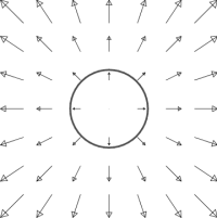
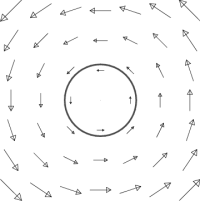
Can we use these ideas to investigate graphically the divergence and curl of a given vector field? Consider the two vector fields above. In case case, can you find the divergegence? The ($\kk$-component of the) curl?
A natural place to start is at the origin. So draw a small box around the origin. 1) Is there circulation around the loop? Is there flux across the loop?
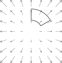
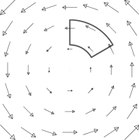
The figures above help us determine the divergence and curl at the origin, but not elsewhere. The divergence is a function, and the curl is a vector field, so both can vary from point to point. We therefore need to examine loops which are not at the origin. It is useful to adapt the shape of our loop to the vector field under consideration. Both of our vector fields are better adapted to polar coordinates than to rectangular, so we use polar boxes. Can you determine the divergence and ($\kk$-component of the) curl using the loops below? Imagine trying to do the same thing with a rectangular loop, or even a circular loop.
Finally, it is important to realize that not all vector fields which point away from the origin have divergence, and not all vector fields which go around the origin have curl. The two examples below demonstrate this important principle; they have no divergence or curl away from the origin. These examples represent solutions of Maxwell's equations for electromagnetism. The figure on the left describes the electric field of an infinite charged wire; the figure on the right describes the magnetic field due to an infinite current-carrying wire (with current coming out of the page at the origin).


1)
In two dimensions, both “boxes” are loops. In three dimensions, the
oriented box used to measure circulation is still a loop, but the box used to
measure flux is now an ordinary, 3-dimensional box.