• This is a group assignment: please form your groups in CANVAS. Group size should be at most 3 for this assignment.
• Your group should keep a journal in CANVAS (Google Docs format). Please state who are the members. In the journal: document your progress, state the issues, and pose questions to me, if any.
• THE FIRST JOURNAL ENTRIES ARE DUE BY TUESDAY 2/7
• I can help you to move forward and/or get off the ground in the lab meetings and by communication through CANVAS. I will respond by email or by making notes in the files.
• You should prepare for the lab ahead of the time:
  • know how to download, unpack the software, and run the demos
• Turn in PARTS 2 and 4. Part 3 is required for those (advanced students) who choose not to use ACF, it is extra credit for others.
• The end product of this assignment should be a report in PDF in which you describe what you did and how you completed the project (Parts 2 and 4). You should properly acknowledge and quote all the necessary sources. Show me the image of the mesh, and the code (upload to CANVAS in one PDF file).
• THE REPORT IS DUE BY MONDAY 2/13

The journal articles written by the authors of the code(s) that are provided in CANVAS, or are available online as below.

1. Create a grid over the unit square Unit=[-1,1]x[-1,1],
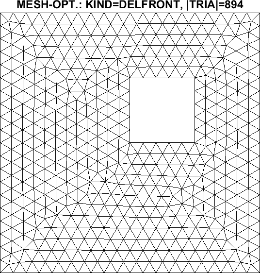
2. create a grid over the region RminusR (a rectangle from which another rectangle was taken out) shown in the image

   

• DISTMESH written by Olof Persson (SIAM Review paper in CANVAS),

  You can start with meshdemo2d or with examples on the distmesh website. Also, try these below.
  To create a grid over Unit, use
  >> fd = @(p)(drectangle(p,0,1,0,1));
  >> [p,t]=distmesh2d(fd,@huniform,0.5,[-1,-1; 1,1],[0,0;0,1;1,0;1,1]);
  Alternatively, use
  >> pv = [-1 -1; -1 1; 1 1; 1 -1; -1 -1];
  >> [p,t]=distmesh2d(@dpoly,@huniform,0.1,[-1,-1; 2,1],pv,pv);
  To create a grid over RminunsR region you can use
  >>fd=@(p) ddiff(drectangle(p,-1,1,-1,1),drectangle(p,0,0.5,0,0.5));
  >>[p,t]=distmesh2d(fd,@huniform,0.1,[-1,-1;1,1],[]);
  (As you see this may not work so well. Modify the code to get the output right)

• MESH2D extends distmesh so you can mesh a region defined by its boundary.

  See github mesh2d or Matlab File Exchange mesh2d.
  You can start with tridemo(5). Or, use a script and example mesh which I wrote based on tridemo.m. See demoMP.m and the mesh file RminusR.msh.

If (A) is too easy, do (B)

(A): Create a grid/mesh (triangulation, quadrangulation) Τ_h over the blue region RminusCircles Ω shown in the image.

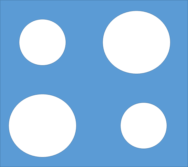
The square should be [-1,1]x[-1,1]; the small circles should have radius 0.3, and the large circles should have radius=0.4. The centers of the circles can be at (+/-0.5,+/-0.5) or elsewhere chosen by you so that the circles do not overlap. (Or, make them overlap for extra credit).

Extra: Create a grid over the entire unit square (without excluding the circles) so that the white circular regions have a refined grid on them.

(B): Create a grid over some other region that is important in your research area, and which is at least as complex as the one in (A). (For example, river channel, mechanical tool, cross-section through a sand layer. It would be good for this region to be non-convex and/or to have holes).

1. ACF code (MATLAB). (Paper by Alberty, Carstensen, Funken in CANVAS), See also the website of C. Carstensen ACF and other software, some of which includes mixed method solvers for elasticity and viscoelasticity.
2. IFISS software (MATLAB) (SIAM Review paper in CANVAS). See also the website IFISS. Find the demos: diff_testproblem for navier_testproblem
3. MFEM (C++ library) MFEM website
4. dealII (C++ library) dealII website
5. FeniCS (Python and C++ interfaces) FEniCS website

• what type of grid/elements it uses (simplicial, rectangular), (P₁, Q₁, quadratics, ...)
• what platform does it run on (Windows, Linux,...)
• what language is it written in and how to modify it
• what is the output it produces (text files, VTK format, ...)
• what do the demo examples solve (diffusion, Stokes, ...)
• what are the major references, URL etc.
• how easy is it to modify the code to include extra output, variable coefficients etc.
• what are the special features (error estimates, adaptivity, solvers, ...)

(A) -Δ u=1, with homogeneous Dirichlet boundary conditions on the entire boundary.

(B) -Δ u=1, with boundary conditions u(-1,y)=1,u(1,y)=0, and homogeneous Neumann conditions on the remaining boundary.

Each FE solver needs a file with some information about a grid, in a particular format (the principles are similar, the details vary). It also needs you to assign the boundary conditions, and provide the code for the load vector etc.

If you are interested in working with DISTMESH or MESH2D for meshing, and ACF for FE solver, read on.

• MESH2D and DISTMESH produces a list of points p and of triangular elements t (in MESH2D demos they are called vert and tria).
• ACF code needs the files coordinates.dat and elements3.dat. These are easy to create from p and t (write them to a file).
• ACF also needs a list of boundary nodes so you can produce dirichlet.dat and neumann.dat. This step is tedious to do by hand.

  I wrote a piece of code mesh2acf.m to assist in this. The code checks the orientation of triangles, warns the user if the elements are degenerate, extracts boundary nodes etc., and saves p and t in an appropriate format. (The code also does uniform mesh refinement, if needed).

• Next you need to make sure you encode the problem data (right hand side=load, and Dirichlet and/or Neumann data) correctly.