1. Introduction

Lie algebras are classified using Dynkin diagrams, which encode the geometric structure of root and weight diagrams associated with an algebra. This paper begins with an introduction to Lie algebras, roots, and Dynkin diagrams. We then show how Dynkin diagrams define an algebra's root and weight diagrams, and provide examples showing this construction. In Section $3$, we develop two methods to analyze subdiagrams. We then apply these methods to the exceptional Lie algebra $F_4$, and describe the slight modifications needed in order to apply them to $E_6$. We conclude by listing all Lie subalgebras of $E_6$.

2. Root and Weight Diagrams of Lie Algebras

We summarize here some basic properties of root and weight diagrams. Further information can be found in [1], [2], and [3]. A description of how root and weight diagrams are applied to particle physics is also given in [2].

2.1 Lie Algebras

A Lie algebra $g$ of dimension $n$ is an $n$-dimensional vector space along with a product $[\ ,\ ]$:$ g \times g \to g$, called a commutator, which is anti-commutative ($[x,y] = -[y,x]$) and satisfies the Jacobi Identity $$[x,[y,z]] + [y,[z,x]] + [z,[x,y]] = 0$$ for all $x,y,z \in g$. A Lie algebra is called simple if it is non-abelian and contains no non-trivial ideals. All complex semi-simple Lie algebras are the direct sum of simple Lie algebras. Thus, we follow the standard practice of studying the simple algebras, which are the building blocks of the semi-simple algebras.

There are four infinite families of Lie algebras as well as five exceptional Lie algebras. The (compact, real forms of) the algebras in the four infinite families correspond to special unitary matrices (or their generalizations) over different division algebras. The algebras $B_n$ and $D_n$ correspond in this way to real special orthogonal groups in odd and even dimensions, $SO(2n+1)$ and $SO(2n)$, respectively. The algebras $A_n$ correspond to complex special unitary groups $SU(n+1)$, and the algebras $C_n$ correspond to unitary groups $SU(n,\mathbb{H})$ over the quaternions, which are more usually described as (some of the) symplectic groups.

While Lie algebras are usually classified using their complex representations, there are particular real representations, based upon the division algebras, which are of interest in particle physics. Manogue and Schray [4] describe the use of quaternions $\mathbb{H}$ to construct $su(2,\mathbb{H})$ and $sl(2, \mathbb{H})$, which are real representations of $B_2=so(5)$ and $D_3 = so(5,1)$, respectively. As they discuss, their construction naturally generalizes to the octonions $\mathbb{O}$, yielding the real representations $su(2,\mathbb{O})$ and $sl(2,\mathbb{O})$ of $B_4 = so(9)$ and $D_5 = so(9,1)$, respectively. This can be further generalized to the $3 \times 3$ case, resulting in $su(3, \mathbb{O})$ and $sl(3, \mathbb{O})$, which preserve the trace and determinant, respectively, of a $3 \times 3$ octonionic hermitian matrix, and which are real representations of two of the exceptional Lie algebras, namely $F_4$ and $E_6$, respectively [5]. The remaining three exceptional Lie algebras are also related to the octonions [6, 7]. The smallest, $G_2$, preserves the octonionic multiplication table and is $14$-dimensional, while $E_7$ and $E_8$ have dimensions $133$ and $248$, respectively. A major stem in describing the infinite-dimensional unitary representation of the split form of $E_8$ was recently completed by the Atlas Project [8].

In sections $2$ and $3$, we label the Lie algebras using their standard name (e.g. $A_n, B_n$) and also with a standard complex representation (e.g. $su(3)$, $so(7)$). In section $4$, when discussing the subalgebras of $E_6$, we also give particular choices of real representations.

2.2 Roots and Root Diagrams

Every simple Lie algebra $g$ contains a Cartan subalgebra $h \subset g$, whose dimension is called the rank of $g$. The Cartan subalgebra $h$ is a maximal abelian subalgebra such that $ad H$ is diagonalizable for all $H \in h$. The Killing form can be used to choose an orthonormal basis $\{h_{1}, \cdots, h_{l}\}$ of $h$ which can be extended to a basis $$\{ h_{1}, \cdots, h_{l}, g_1, g_{-1}, g_2, g_{-2}, \cdots, g_{\frac{n-l}{2}}, g_{-\frac{n-l}{2}} \} $$ of $g$ satisfying:

Let $\Delta$ denote the collection of non-zero roots. For roots $r^{i}$ and $r^{j} \ne -r^i$, if there exists $r^{k} \in \Delta$ such that $r^i + r^j = r^k$, then the associated operators for $r^i$ and $r^j$ do not commute, that is, $[ g_i, g_j ] \ne 0$. In this case, $[g_i, g_j] = C^{k}_{ij}g_{k}$ (no sum), with $C^k_{ij} \in \mathbb{C}, C^i_{ij} \ne 0$. If $r^i + r^j \not\in \Delta$, then $[g_i, g_j] = 0$.

When plotted in $\mathbb{R}^l$, the set of roots provide a geometric description of the algebra. Each root is associated with a vector in $\mathbb{R}^l$. We draw $l$ zero vectors at the origin for the $l$ zero roots corresponding to the basis $h_1, \cdots, h_l$ of the Cartan subalgebra. For the time being, we then plot each non-zero root $r^i = \langle\lambda_1^i, \cdots, \lambda_l^i\rangle$ as a vector extending from the origin to the point $\langle\lambda_1^i, \cdots, \lambda_l^i\rangle$. The terminal point of each root vector is called a state. As is commonly done, we use $r^i$ to refer to both the root vector and the state. In addition, we allow translations of the root vectors to start at any state, and connect two states $r^i$ and $r^j$ by the root vector $r^k$ when $r^k + r^i = r^j$ in the root system. The resulting diagram is called a root diagram.

As an example, consider the algebra $su(2)$, which is classified as $A_1$. The algebra $su(2)$ is the set of $2 \times 2$ complex traceless Hermitian matrices. Setting

1. $[h_1, h_1] = 0$
2. $[h_1, g_1] = 1 g_1$
3. $[h_1, g_{-1}] = -1 g_{-1}$
4. $[g_{1}, g_{-1}] = h_1$

Figure 1. Root Diagram of $A_1 = su(2)$

2.3 Weights and Weight Diagrams

An algebra $g$ can also be represented using a collection of $d \times d$ matrices, with $d$ unrelated to the dimension of $g$. The matrices corresponding to the basis $h_1, \cdots, h_l$ of the Cartan subalgebra can be simultaneously diagonalized, providing $d$ eigenvectors. Then, a list $w^m$ of $l$ eigenvalues, called a weight, is associated with each eigenvector. Thus, the diagonalization process provides $d$ weights for the algebra $g$. The roots of an $n$-dimensional algebra can be viewed as the non-zero weights of its $n \times n$ representation.

Weight diagrams are created in a manner comparable to root diagrams. First, each weight $w^i$ is plotted as a point in $\mathbb{R}^l$. Recalling the correspondence between a root $r^i$ and the operator $g^i$, we draw the root $r^k$ from the weight $w^i$ to the weight $w^j$ precisely when $r^k + w^i = w^j$, which at the algebra level occurs when the operator $g^k$ raises (or lowers) the state $w^i$ to the state $w^j$.

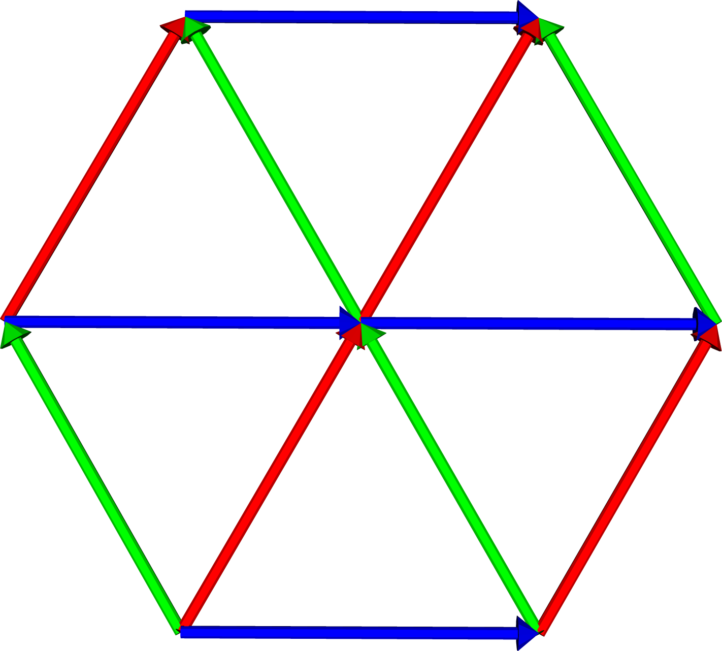
The root and minimal non-trivial weight diagrams of the algebra $A_2 = su(3)$ are shown in Figure 2.¹ The algebra has three pairs of root vectors, which are oriented east-west (colored blue), roughly northwest-southeast (colored red), and roughly northwest-southeast (colored green). The algebra's rank is the dimension of the underlying Euclidean space, which in this case is $l=2$, and the number of non-zero root vectors is the number of raising and lowering operators. The minimal weight diagram contains six different roots, although we've only indicated one of each raising and lowering root pair. Using the root diagram, the dimension of the algebra can now be determined either from the number of non-zero roots or from the number of root vectors extending in different directions from the origin. Both diagrams indicate that the dimension of $A_2 = su(3)$ is $8 = 6+2$. A complex semi-simple Lie algebra can almost² be identified by its dimension and rank. We note that the algebra's root system, and hence its root diagram or weight diagram, does determine the algebra up to isomorphism.

Figure 2. Root and Minimal Weight Diagrams of $A_2=su(3)$

2.4 Constructing Root Diagrams from Dynkin Diagrams

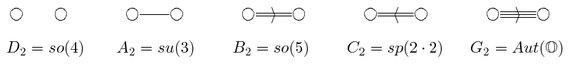
In 1947, Eugene Dynkin simplified the process of classifying complex semi-simple Lie algebras by using what became known as Dynkin diagrams [9]. As pointed out above, the Killing form can be used to choose an orthonormal basis for the Cartan subalgebra. Then every root in a rank $l$ algebra can be expressed as an integer sum or difference of $l$ simple roots. Further, the relative lengths and interior angle between pairs of simple roots fits one of four cases. A Dynkin diagram records the configuration of an algebra's simple roots.

Each node in a Dynkin diagram represents one of the algebra's simple roots. Two nodes are connected by zero, one, two, or three lines when the interior angle between the roots is $\frac{\pi}{2}$, $\frac{2\pi}{3}$, $\frac{3\pi}{4}$, or $\frac{5\pi}{6}$, respectively. If two nodes are connected by $n$ lines, then the magnitudes of the corresponding roots satisfy the ratio $1:\sqrt{n}$. An arrow is used in the Dynkin diagram to point toward the node for the smaller root. If two roots are orthogonal, no direct information is known about their relative lengths.

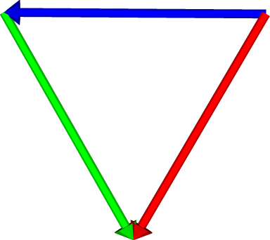
We give the Dynkin diagrams for the rank $2$ algebras in Figure 3 and the corresponding simple root configurations in Figure 4. For each algebra, the left node in the Dynkin diagram corresponds to the root $r^1$ of length $1$, colored red and lying along the horizontal axis, and the right node corresponds to the other root $r^2$, colored blue.

Figure 3. Rank 2 Dynkin Diagrams

$D_2 = so(4)$	$A_2 = su(3)$	$B_2 = so(5)$	$C_2 = sp(2\cdot 2)$	$G_2 = Aut(\mathbb{O})$
Figure 4. Rank 2 Simple Roots

In $\mathbb{R}^l$, each root $r^i$ defines an $(l-1)$-dimensional hyperplane which contains the origin and is orthogonal to $r^i$. A Weyl reflection for $r^i$ reflects each of the other roots $r^j$ across this hyperplane, producing the root $r^k$ defined by $$r^k = r^j - 2(\frac{r^j {\tiny \bullet} r^i}{|r^i|})\frac{r^i}{|r^i|} $$ According to Jacobson [1], the full set of roots can be generated from the set of simple roots and their associated Weyl reflections.

We illustrate how the full set of roots can be obtained from the simple roots using Weyl reflections in Figure 5. We start with the two simple roots for each algebra, as given in Figure 4. For each algebra, we refer to the horizontal simple root, colored red, as $r^1$, and the other simple root, colored blue, as $r^2$. Step $1$ shows the result of reflecting the simple roots using the Weyl reflection associated with $r^1$. In this diagram, the black thin line represents the hyperplane orthogonal to $r^1$, and the new resulting roots are colored green. Step $2$ shows the result of reflecting this new set of roots using the Weyl reflection associated with $r^2$. At this stage, both $D_2 = so(4)$ and $A_2 = su(3)$ have their full set of roots. We repeat this process again in steps 3 and 4, using the Weyl reflections associated first with $r^1$ and then with $r^2$. The full root systems for $B_2 = so(5)$ and $C_2 = sp(2\cdot 2)$ are obtained after the three Weyl reflections. Only $G_2$ requires all four Weyl reflections.

$D_2 = so(4)$		$A_2 = su(3)$		$B_2=so(5)$		$C_2=sp(2\cdot 2)$		$G_2 = Aut(\mathbb{O})$
Figure 6. Root Diagrams of Simple Rank $2$ Algebras

The full set of roots have been produced once the Weyl reflections fail to produce additional roots. The root diagrams are completed by connecting vertices $r^i$ and $r^j$ via the root $r^k$ precisely when $r^k + r^i = r^j$. From the root diagrams in Figure 6, it is clear that the dimension of $A_2=su(3) \textrm{ is }8$ and the dimension of $G_2 \textrm{ is }14$, while both $B_2=so(5)$ and $C_2=sp(2\cdot 2)$ have dimension $10$. Further, since the diagram of $B_2$ can be obtained via a rotation and rescaling of the root diagram for $C_2$, it is clear that $B_2$ and $C_2$ are isomorphic.

2.5 Constructing Weight Diagrams from Dynkin Diagrams

Root diagrams are a specific type of weight diagram. While the states and roots can be identified with each other in a root diagram, this does not happen for general weight diagrams. Weight diagrams are a collection of states, called weights, and the roots are used to move from one weight to another. Although it has only one root diagram, an algebra has an infinite number of weight diagrams.

Like a root diagram, any one of an algebra's weight diagrams can be constructed entirely from its Dynkin diagram. The Dynkin diagram records the relationship between the $l$ simple roots of a rank $l$ algebra. Each simple root $r^1, \cdots, r^l$ is associated with a weight $w^1, \cdots, w^l$. When all integer linear combinations of these weights are plotted in $\mathbb{R}^l$, they form an infinite lattice of possible weights. This lattice contains every weight from every $d \times d$ $(d \ge 0)$ representation of the algebra. These weights may be ordered. Every weight diagram then contains a highest weight $W$ which satisfies $W > W_i$ for every other weight $W_i$ in the diagram. Alternatively, a diagram's highest weight $W$ is an element of the boundary $\overline{W}$ of the set of all weights in the diagram; $\overline{W}$ contains all the weights in the diagram which are furthest from the origin. A particular weight diagram is chosen by selecting a weight $W$. Weyl reflections related to the weights $w^1, \cdots, w^l$ determine the weights in $\overline{W}$ for the weight diagram. To determine the diagram's weights in the interior of $\overline{W}$, we note that valid weights must be connected by the algebra's roots. Hence, all of the weights within $\overline{W}$ which are integer linear combinations of the roots away from the weights in $\overline{W}$ are valid and should be a part of the diagram. Having selected all of the diagram's valid weights, we complete the diagram by connecting pairs of weights with root vectors.³ Choosing a new weight $W$ outside the original weight diagram's boundary $\overline{W}$ selects a new, larger, weight diagram. A smaller weight diagram is created by selecting a weight contained in the interior of $\overline{W}$.

An equivalent method [10] constructs weight diagrams while avoiding the explicit use of Weyl reflections. First, the $l$ simple roots $r^1, \cdots, r^l$ are used to define the Cartan matrix $A$, whose components are $a_{ij} = 2 \frac{r^i {\tiny \bullet} r^j}{r^i {\tiny \bullet} r^i}$. Equivalently, the components are: \[ a_{ij} =\begin{cases} 2, &\text{if $i = j$;}\\ 0, &\text{if $r^i$ and $r^j$ are orthogonal;}\\ -3, &\text{if the interior angle between $r^i$ and $r^j$ is $\frac{5\pi}{6}$, and $\sqrt{3}|r^i| = |r^j|$;}\\ -2, &\text{if the interior angle between roots $r^i$ and $r^j$ is $\frac{3\pi}{4}$, and $\sqrt{2}|r^i| = |r^j|$;}\\ -1, &\text{in all other cases;}\\ \end{cases} \]

Cartan matrices are invertible. Thus, the fundamental weights $w^1, \cdots, w^l$ defined by \[w^i = \sum_{k=1}^{l}(A^{-1})_{ki}r^k\] are linearly independent. We create an infinite lattice $\mathbb{W} = \{ m_i w^i | m_i \in \mathbb{Z}\}$ of possible weights in $\mathbb{R}^l$, and then label each weight $W^i = m^i_j w^j \in \mathbb{W}$ using the $l$-tuple $M^i = \left[m^i_1, \cdots, m^i_l\right]$, called a mark. We choose one of the infinite number of weight diagrams by specifying $l$ non-negative integers $m^0_1, \cdots, m^0_l$ for the mark of the highest weight $W^0$.

While the components of the Cartan matrix record the geometry of the simple roots, the components of each mark record the geometric configuration of the weights within the lattice. Each weight $W^i$ is part of a shell of weights $\overline{W}$ which are equidistant from the origin. As discussed earlier, Weyl reflections associated with the fundamental weights can be used to find the weights in $\overline{W}$. The diagram's entire set of valid weights can also be determined using the mark $M^i$ of each weight. The positive integers $m^i_j \in M^i$ list the maximum number of times that the simple root $r^j$ can be subtracted from $W^i$ while keeping the new weights on or within the boundary $\overline{W}$. Thus, weights $W^i - 1 r^j, \cdots, W^i - (m^i_j) r^j \textrm{ (no sum)}$ are valid weights occurring on or inside $\overline{W}$. These new weights have marks $M^i - A_i^{\it{T}}, M^i - 2 A_i^{\it{T}}, \cdots, M^i - m^i_j A_i^{\it{T}}$, where $A_i^{\it{T}}$ is the transpose of the $i$th column of the Cartan matrix $A$. Thus, given a weight diagram's highest weight $W^0$, this procedure selects all of the diagram's weights from the infinite lattice. The diagram is completed by connecting any two weights $W^i$ and $W^k$ by the root $r^j$ whenever $W^i + r^j = W^k$.

This procedure is carried out for the the algebra $B_3=so(7)$, whose simple roots are \[ \begin{array}{ccc} r^1 = \langle\sqrt{2},0,0\rangle, & r^2 = \langle-\sqrt{\frac{1}{2}}, -\sqrt{\frac{3}{2}}, 0\rangle, & r^3 = \langle0, \sqrt{\frac{2}{3}}, \sqrt{\frac{1}{3}}\rangle \end{array} \] We produce the Cartan matrix $A$, find $A^{-1}$, and list the fundamental weights.

Starting with the highest weight $W^0 = w^1$, whose mark is $\left[1,0,0\right]$, the above procedure generates the following weights:

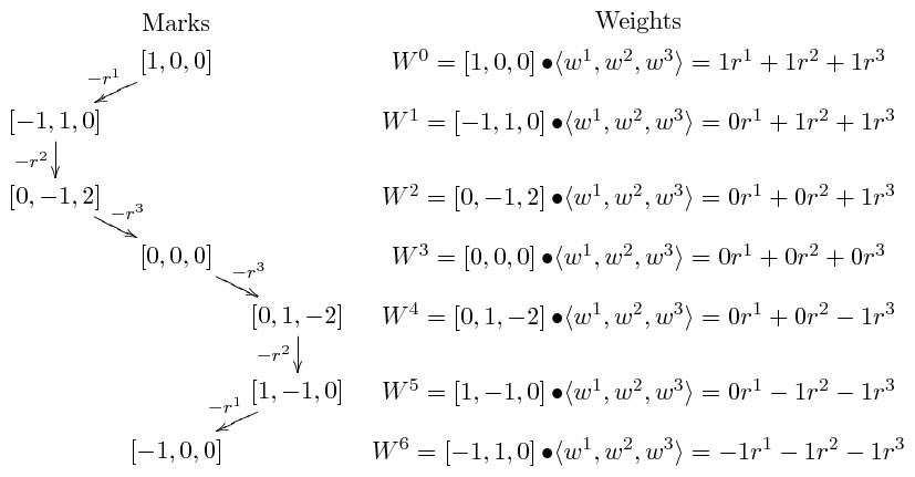
We plot the weight $W^0, \cdots, W^6$ and the appropriate lowering roots $-r^1, \cdots, -r^3$ at each weight for this weight diagram of $B_3 = so(7)$ in Figure 7. The full set of roots are used to connect pairs of weights, giving the complete weight diagram of $B_3 = so(7)$ in Figure 8.

2.6 Rank 3 Root and Weight Diagrams

Using the procedures outlined above, we catalog the root and minimal weight diagrams for the rank $3$ algebras. We did this by writing a Perl program to generate the weight and root diagram structures and return executable Maple code. We then used Maple and Javaview to display the pictures.

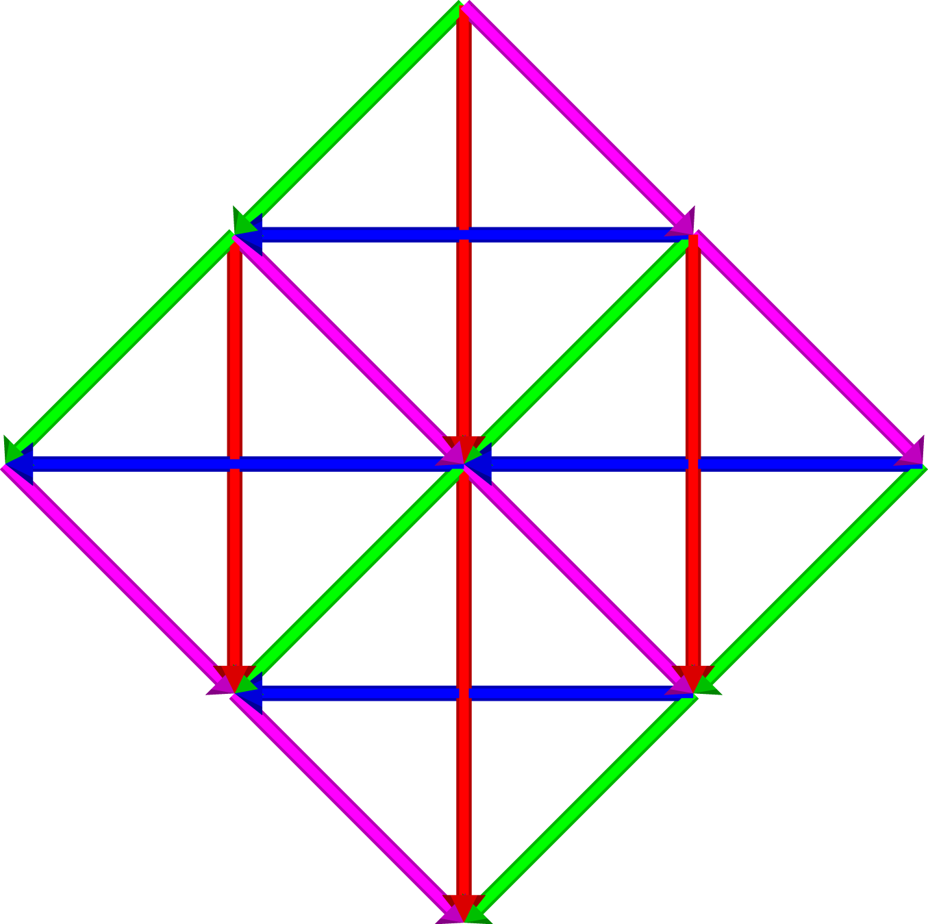
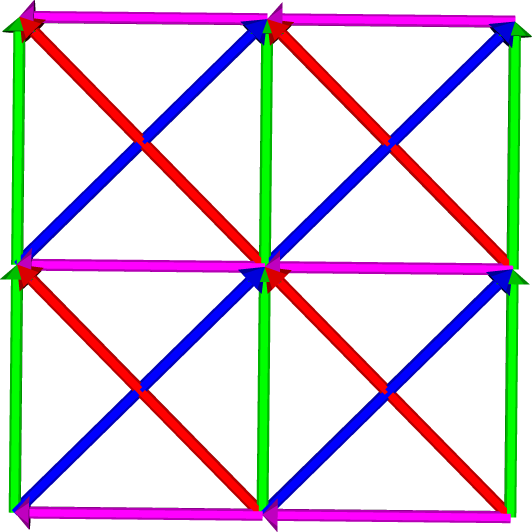
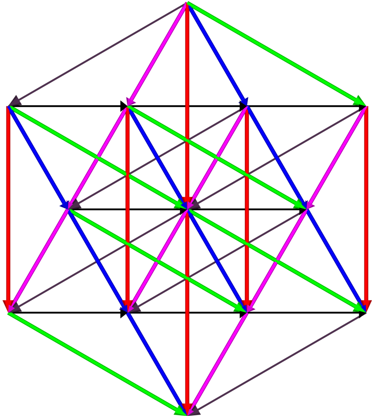
The $3$-dimensional root diagrams of the rank $3$ algebras are given in Figure 9. The root diagrams of $A_3=su(4)$ and $D_3=so(6)$ are identical. Hence, $A_3 = D_3$. These algebras have dimension $15$, as their root diagram contains $12$ non-zero states. The $B_3=so(7)$ and $C_3=sp(2\cdot 3)$ algebras both have dimension $21$, and their root diagrams each contain $18$ non-zero states. Each of these algebras contain the $A_2=su(3)$ root diagram, which is a hexagon. This can be seen at the center of each rank $3$ algebra by turning its root diagram in various orientations. The modeling kit ZOME [11] can be used to construct the rank $3$ root diagrams. The kit contains connectors of the right length and nodes with the correct configuration of connection angles to construct all of the rank $3$ root diagrams.

An algebra's minimal weight diagram has the fewest number of weights while still containing all of the roots. Figure 10 shows the minimal weight diagrams for $A_3=D_3$, $B_3$, and $C_3$. Each root occurs once in the diagram for $A_3=D_3$, while in the diagram for $B_3$ every root is used twice. The minimal weight diagram for $C_3$ is centered about the origin, and the roots passing through the origin (colored red, blue, and brown) occur once, while the other roots occur twice.

Go to Subalgebras of Algebras

²For algebras of rank $6$ and lower, the exceptions are that $B_n = so(2n+1)$ and $C_n=sp(2\cdot n)$ have the same dimension for each rank $n$, and that $B_6$, $C_6$, and $E_6$ all have dimension $78$.

³The distance between adjacent weights in the infinite lattice is less than or equal to the length of each root vector. Root vectors do not always connect adjacent weights, but often skip over them.